How to Create a Budget Using Microsoft Excel
by BrendanK28 in Living > Organizing
735 Views, 4 Favorites, 0 Comments
How to Create a Budget Using Microsoft Excel
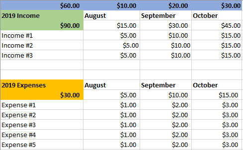
Microsoft Office comes with a lot of useful applications including Microsoft Word, PowerPoint, Excel, and Access. Most people use Microsoft Word and PowerPoint due to them being user friendly. It’s useful to know how to use Microsoft Excel even though it’s not the most user-friendly program. Excel is a unique application that allows user to create mathematical formulas and convert those formulas into charts once the numbers are entered. Using Microsoft Excel is no easy task, but the following instructions will guide you step by step how to create a budget using Microsoft Excel.
** Before we have you jump into Microsoft Excel, let us introduce to you some terms that are most common with Microsoft Excel. **
Supplies
A Computer
Microsoft Excel
A list of monthly expenses and income

This is a cell. This is where you will type your data. Keep in mind that you can make the cell bigger or smaller so it can fit all your data.

This is called the “Name Box”. This will show you what cell you are working in. Look at the screenshot below for reference.

This is the formula bar. This bar will show you what text or formula is entered in the specific cell that was selected
This will be useful to remember throughout the instructions. IF the text that is entered in a cell is spilling over into the other cell, double-click the middle of both cell columns. This will re-size the column to fit all the text.
Let’s get started!
Click on the Microsoft Excel icon on your computer and then open a blank spreadsheet. Keep in mind that the icon might be slightly different if you are using a Mac computer.

First thing first is to highlight cell A1 all the way to cell D1. Once Highlighted make the cell Blue by selecting the color option at the top bar.

Then in cell A2, type “2019 Income”

In cell A3, type “$0.00”. Don’t worry, we’ll go back and enter your actual data when we go further into the instructions.

Highlight cell A2 and A3 and set them to the color Green, or any variant of green that you prefer.

Please enter the names of the past 3 months starting from cell B2 to cell D2. You’ll be able to add more months to the budget if needed later.

We know everyone has a different number of sources for income, but for these instructions let’s just put “Income #1” in cell A4, “Income #2” in cell A5, and “Income #3” in cell A6.

Next step is to enter “$0.00” in the cells B4 to B6. Do the same in C4 to C6 and D4 to D6. Your screen should look like the screenshot above.

Now it’s time to create the expenses for the budget. In cell A9, type “2019 Expenses”. Right below it, in cell A10, type “$0.00”. Once the number has been entered, highlight cell A9 and A10 and add an Orange color to it.

Type “Expense #1” in cell A11 and continue your way down all the way to A15. Make sure to increase the “Expense#” by one. See screenshot above for reference.
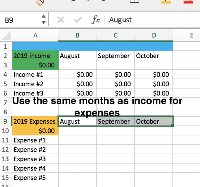
Enter the same months that you entered in cells B2 to D2 in the cells B9 to D9

Enter “$0.00” in cells B11 to B15. Do the same for cells C11 to C15 and D11 to D15.

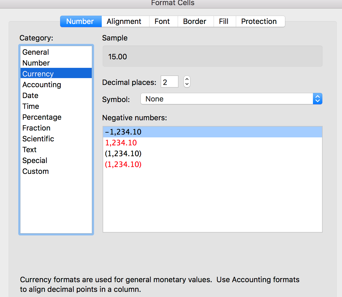
Now it’s time to make sure that we set the Number Format to Currency. This will make sure that the cells remain in currency if there is a change. Highlight cells B3 all the way to cell D6. Right-click and select “Format Cells”. A new window will appear after that. In the new window, select “Currency”. Make sure the decimal place is set to 2, and then click Okay. Make sure we also set the Currency format in cell A3.

Follow the same steps that you did in Step #16 but this time do it for cells B10 all the way to D15. Don’t forget to apply the Currency Format in cell A10.
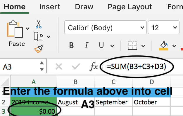
Now it’s time to create the formulas. Click on cell A3 and type in “=SUM(B3+C3+D3)”. This will add the 3 cells and put the total in Cell A3.
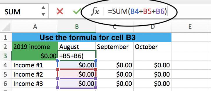
Now, lets add the income for each month. Click on cell B3 and type “=SUM(B4+B5+B6)”. This will add the numbers in those cells and place the total in B3.

Now that the first month is complete, let’s move on to the next. Click on cell C3 and type “=SUM(C4+C5+C6)”. This will add the numbers in those cells and place the total in cell C3.
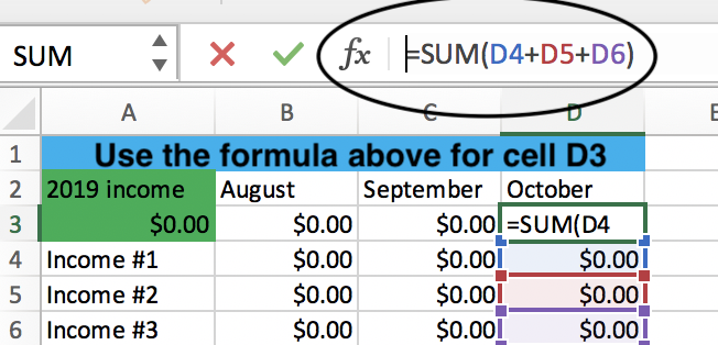
Now on to the next month, click on cell D3 and type “=SUM(D4+D5+D6)”. This will also add the numbers in those cells and add the total in cell D3.

Let’s move on to the expense section. Select cell A10 and type in “=SUM(B10+C10+D10)”. This will add the total of the 3 months to cell A10.

Now it’s time to add the expenses for each month. Select cell B10 and type “=SUM(B11+B12+B13+B14+B15)”.

Let’s move on to the next month. Select cell C10 and type “=SUM(C11+C12+C13+C14+C15)”.

Let’s move on to the last month. Select cell D10 and type “=SUM(D11+D12+D13+D14+D15)”.


Click on B1 and enter the formula “=SUM(B3 – B10)”. This shows the actual income for that month after all expenses have been paid. Now click on C1 and enter the formula “=SUM(C3 – C10)”. Lastly, click on D1 and enter the formula “=SUM(D3 – D10)”.

Click on A1 and type the formula “=SUM(A3-A10)”. This will provide the income of all the months combined.
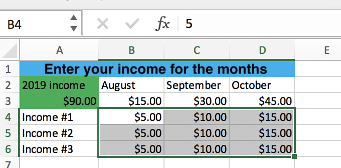
Now it’s time to enter your actual data. Replace the “Income #” text with the name of your job(s).
Budget is Complete!
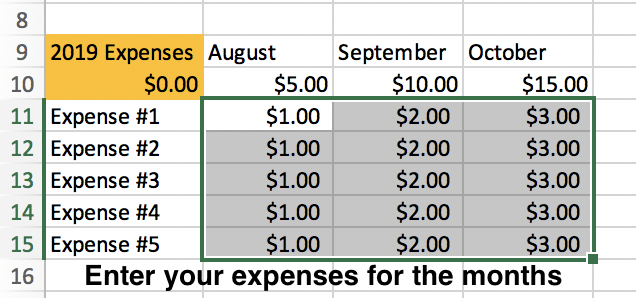
Enter the actual amount of money that you make in the income section based on the month and income. Do the same with the Expense section. Once you have all your information entered, the formulas will do all of the math and properly display how much money you made, spent and have left over in those months. Feel free to customize your budget if needed. Don’t forget to modify the formulas if changes are made.