Learning-Based Lap Time Optimization Using F1TENTH Simulation

Ever wondered how autonomous racecars learn to drive smarter, not just faster? This project dives into the world of lap time optimization within the F1TENTH simulation environment, aiming to teach a simulated car to anticipate turns, adjust speeds, and choose optimal paths—all without relying on complex machine learning algorithms.

Instead, we embrace a data-driven approach. By analyzing the car's performance—its speed, steering angles, and the curvature of the track—we iteratively refine its trajectory and speed profile. This method mirrors how real-world drivers and engineers use telemetry data to enhance performance.

Whether you're a robotics enthusiast, an aspiring engineer, or someone curious about the mechanics behind autonomous racing, this guide will walk you through building a smarter, more efficient racecar in simulation. Let's embark on this journey of teaching machines to race with finesse.

This project is entirely simulation-based, which means no soldering irons or LiPo batteries — just a laptop and a few key software tools. Here's everything you'll need to follow along:

Software & Frameworks:

1. Python 3.8+ – Our main language for scripting and simulation logic
2. F1TENTH Gym – A lightweight Python-based simulator for autonomous racing
3. → GitHub: f1tenth/f1tenth_gym
4. NumPy + Matplotlib – For all the math, data processing, and visualizations
5. Jupyter Notebook (optional) – For interactive debugging and graphing

We’ll be working with the built-in tracks from the F1TENTH Gym repo. You can find them here:

Example tracks: skirk.csv, esp.csv, aut.csv

Hardware & OS Recommendations

1. Any modern laptop or desktop with Python 3.8+ installed
2. Works on Windows, macOS, or Linux, but we recommend using Linux (Ubuntu) for two reasons:
3. If you plan to integrate this with ROS2 later, you’ll already be in a compatible environment
4. Most robotics workflows and F1TENTH extensions are built and tested on Ubuntu

Bonus: If you're planning to deploy this onto an actual Jetson or racecar setup, you'll already be one step ahead with Linux.

Recommended GitHub Repositories

1. F1TENTH Gym Simulator (Official)
2. F1TENTH Racing Repo w/ Controllers (for ROS integration)

In racing — whether it's Formula 1 or F1TENTH — lap time is the ultimate scorecard. The faster your car gets around the track, the better your chances of winning. But shaving seconds off a lap isn’t just about raw speed — it’s about how smartly you navigate the track.

What Does "Lap Time Optimization" Really Mean?

At its core, it's about:

1. Choosing the best possible path (racing line) through the track
2. Controlling speed so that you're fast where you can be, and cautious where you need to be
3. Minimizing unnecessary steering and abrupt changes in velocity

This makes it a multi-objective control problem involving:

1. Path planning (geometry)
2. Speed planning (dynamics)
3. Stability (vehicle control)

Why Is This Non-Trivial?

Because the best racing line isn’t always the shortest. It’s often the smoothest, the one that lets the car maintain higher speeds longer and avoid energy loss due to braking or oversteering.

Imagine two cars:

1. Car A follows the geometric center of the track
2. Car B takes wider entries, hits apexes, and exits fast — like a real driver

Car B almost always wins. That’s the magic of a well-optimized line.

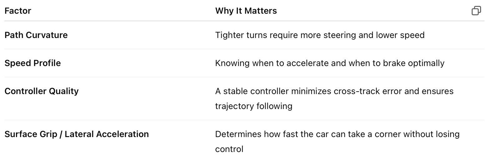
Key Factors That Affect Lap Time

Factor — Why It Matters

Path Curvature — Tighter turns require more steering and lower speed

Speed Profile — Knowing when to accelerate and when to brake optimally

Controller Quality — A stable controller minimizes cross‑track error and ensures trajectory following

Surface Grip / Lateral Acceleration — Determines how fast the car can take a corner without losing control

refer the table from this section above

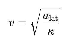
In simulation, we use curvature and maximum lateral acceleration to decide how fast the car can go at each point on the track:

refer the equation from this section above

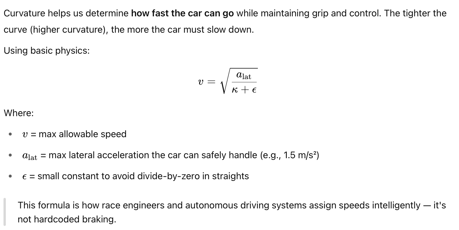
Where:

1. v = speed
2. a_lat = max lateral acceleration the car can handle (based on its dynamics)
3. k = curvature at that point on the path

What This Project Does

This project implements a learning-based pipeline where the system:

1. Starts with a basic path (e.g., midpoints or predefined line)
2. Analyzes curvature and performance
3. Calculates the best speed profile
4. Feeds this into a controller (Pure Pursuit / Stanley)
5. Evaluates and iterates — reducing lap time over time

Want to Dive Deeper? Recommended Reading:

1. “Minimum-Time Trajectory Generation for Quadrotors” – Mellinger & Kumar (2011)
2. “Minimum Time Velocity Planning on a Specified Path” – Verscheure et al.
3. F1TENTH Lecture Notes – Path Planning and Controls

Before we can optimize anything, we need a starting point — a basic trajectory the car can follow around the track. This is often referred to as the baseline path, and it represents what a “non-expert” or default driver might do.

2.1 The Baseline Path

In this project, we use either:

1. A predefined centerline from a track file (skirk.csv, esp.csv, etc.)
2. Or a synthetic path that mimics a simple oval or S-curve if you're building from scratch

These files contain:

1. x, y coordinates of waypoints around the track
2. Sometimes also vx, vy, and speed

You can think of this as the GPS track the car would naïvely follow without optimization.

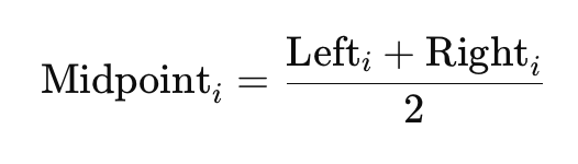
If your track doesn’t have a centerline, you can create one by averaging the left and right boundaries:

refer the equation from this section above

2.2 Initial Controller Setup

To follow this path, we use a path tracking controller. You’ll start with:

Pure Pursuit

1. Looks ahead by a fixed distance (the "lookahead") to find a point on the path
2. Computes the steering angle needed to drive toward that point
3. Very simple, reactive, but struggles in tight turns

Stanley Controller

1. Minimizes two things:
2. Cross-track error (how far off path you are)
3. Heading error (how misaligned you are)
4. More stable at higher speeds, more realistic behavior

You can implement both and compare their behavior — which is exactly what this project does later on.

2.3 Running the First Lap

With the path + controller set up:

1. Run the simulation using constant speed (e.g., 2 m/s)
2. Use F1TENTH Gym’s built-in simulation loop
3. Log data:
4. Actual driven (x, y)
5. Speed, steering angles
6. Time taken per lap

This run serves as your first learning iteration.

Code Structure Example:

Output of This Step:

1. A lap time baseline
2. Actual path taken by the car
3. Steering effort, speed vs. position
4. Everything you need to optimize in the next steps

After running the first lap using your baseline controller (Pure Pursuit or Stanley), the car leaves behind something extremely valuable: data.

That data tells us:

1. Where it was fast or slow
2. Where it struggled with sharp turns
3. Where it over- or under-steered

This is where we start teaching the car to drive smarter.

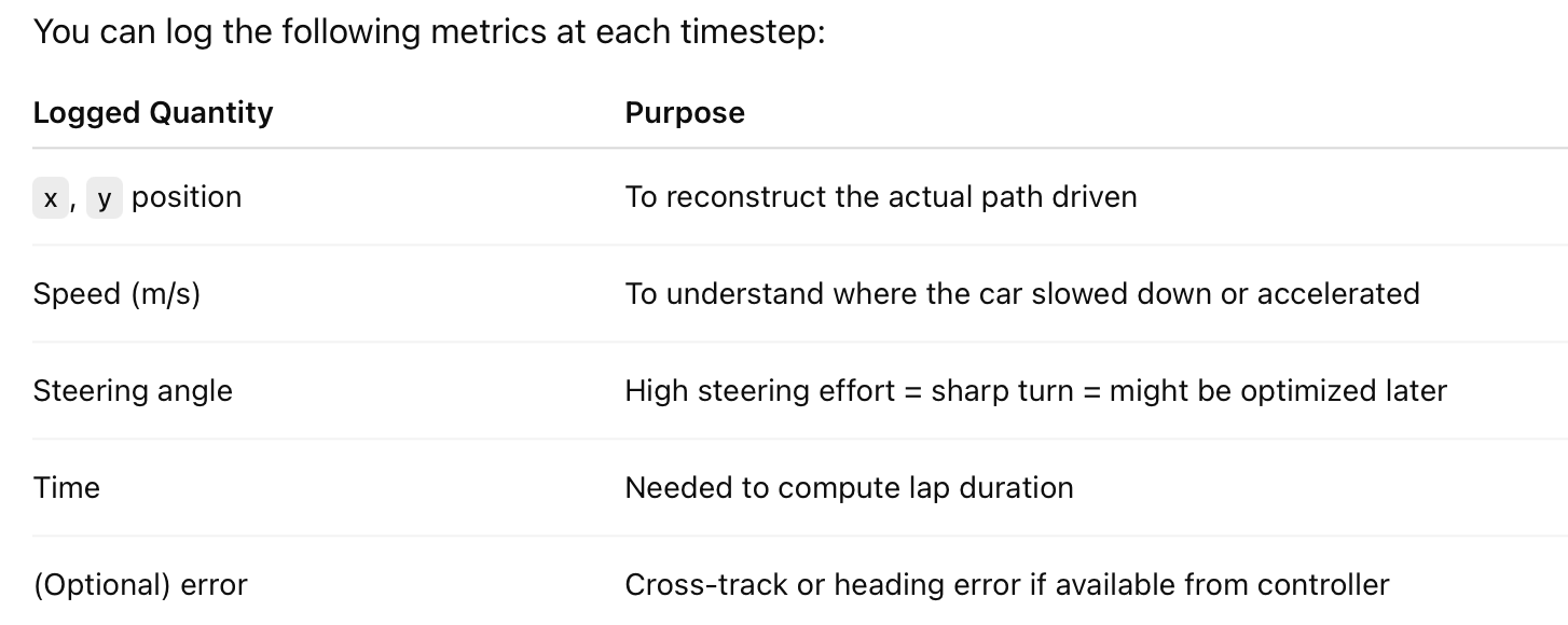
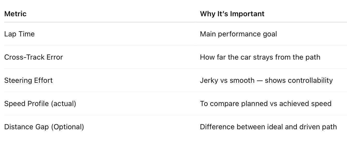
3.1 What We Log From Each Lap

You can log the following metrics at each timestep:

refer the table from this section above

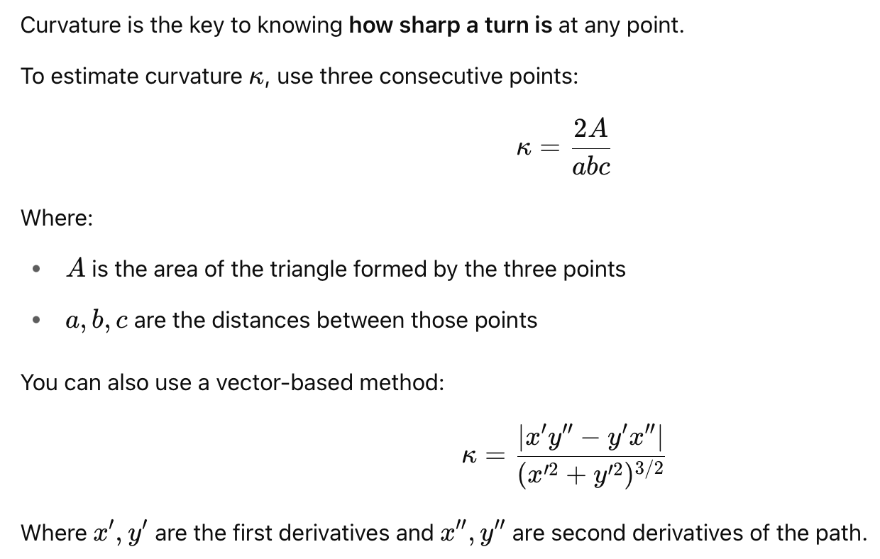
3.2 Computing Curvature from the Path

refer the equation from this section above

3.3 Why Curvature Matters

Curvature helps us determine how fast the car can go while maintaining grip and control. The tighter the curve (higher curvature), the more the car must slow down.

Using basic physics:

refer the equation from this section above

Example Code Snippet (Curvature Calculation):

Output of This Step:

1. You now have a curvature map of the path
2. This helps you generate the optimal speed profile (coming in Step 4!)
3. You've captured all the telemetry needed for learning + optimization

What’s a Speed Profile?

A speed profile assigns a target speed to each point along the trajectory.

It allows the car to:

1. Cruise fast on straights
2. Slow down intelligently before sharp turns
3. Smoothly transition between different speeds

Without it, your controller either uses:

1. A constant speed (too dumb), or
2. Reacts to turns too late (too dangerous)

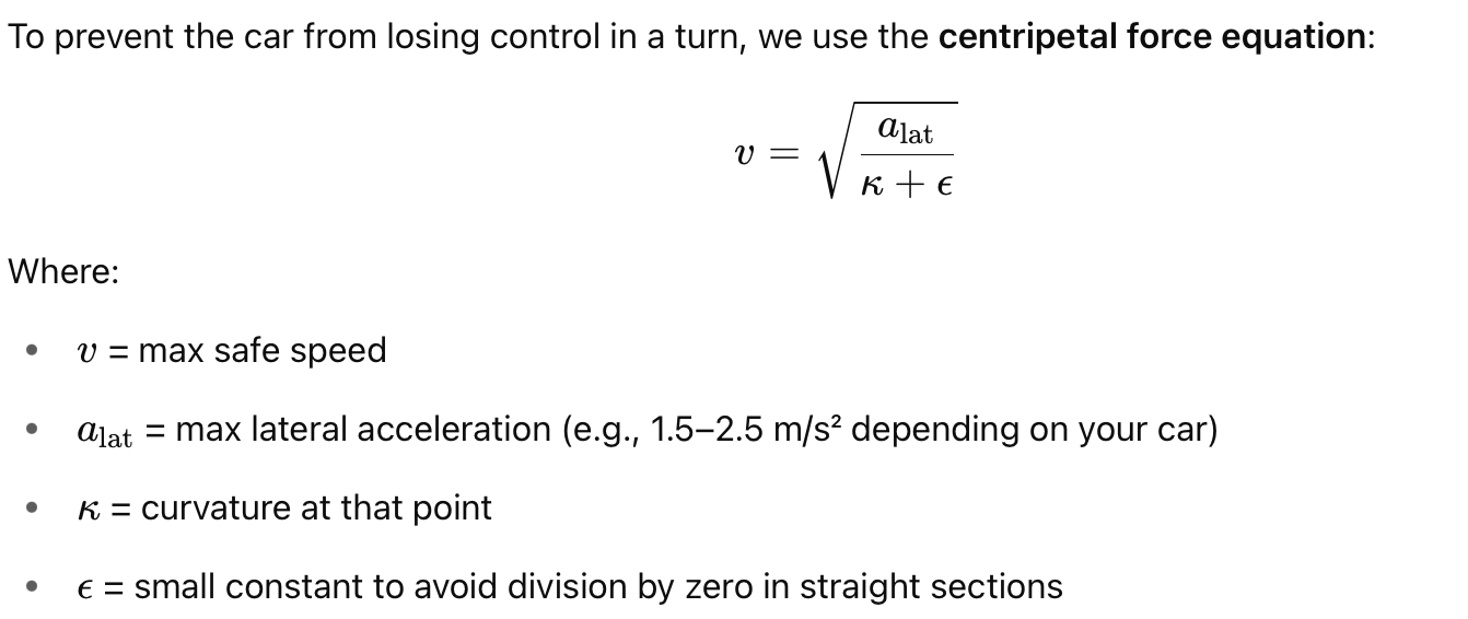
Physics Behind Speed Limiting

To prevent the car from losing control in a turn, we use the centripetal force equation:

refer the table from this section above

Higher curvature → lower max speed

Lower curvature → full throttle

Smoothing the Speed Profile

Raw curvature-based speed may look jagged — and cars hate sudden acceleration or braking.

So we smooth it using a Gaussian filter or spline:

You now have a smooth, safe, and fast speed plan for the whole lap.

Adding Driver Behavior

Want your car to brake before turns or accelerate out of corners?

That comes next — by shifting the speed profile slightly ahead in time so the car anticipates what's coming. You can simulate:

1. Early braking
2. Gradual acceleration zones

This is how we go from a naive robot to a smarter “driver.”

Output of This Step:

1. A smooth array of target speeds, one for each waypoint
2. Realistic, physics-aware driving behavior
3. Ready for simulation using this improved profile

What We Have So Far

You’ve built a smarter trajectory-following system that:

1. Uses an optimized path (baseline or improved)
2. Has a speed profile based on curvature (not hardcoded)
3. Can now run using a controller like Pure Pursuit or Stanley

Now it’s time to simulate and see how well it drives.

Integrating Speed into Your Controller

In your simulation loop:

1. At each timestep, read the target speed for the next waypoint
2. Send this as the velocity command to the car
3. Use your controller (Pure Pursuit or Stanley) to compute the steering angle

If you're using F1TENTH Gym, your loop may look like:

What to Measure

refer the table from this section above

You can now plot:

1. The trajectory: actual vs planned path
2. The speed: profile over time
3. The steering: see where the car overcorrects
4. The lap time: improvement over constant-speed baseline

Now that your car has run a lap using an optimized path and a physics-based speed profile, it’s time to evaluate how well it performed. This is the part where we compare, visualize, and prove that smarter driving leads to better lap times.

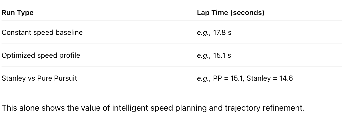
6.1 Lap Time Comparison

The simplest and most impactful metric: How much faster did we get?

refer the table from this section above

6.2 Graphs to Show

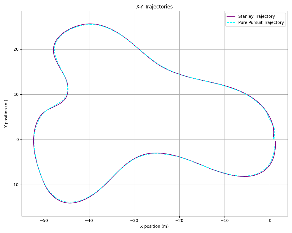
Trajectory Comparison

1. Plot the baseline path vs the actual path driven by each controller
2. Shows tracking accuracy and overall smoothness

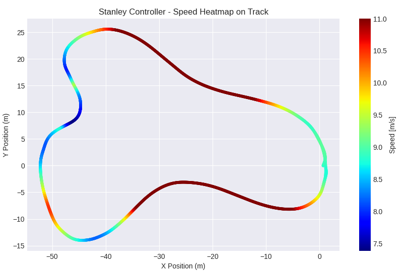
Speed Profile (Planned vs Actual)

1. Shows how closely the car followed the target speed

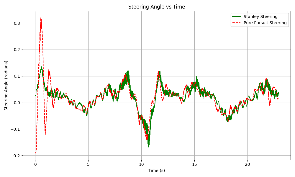
Steering Angle

1. High-frequency zig-zags = poor control
2. Smoother = better handling

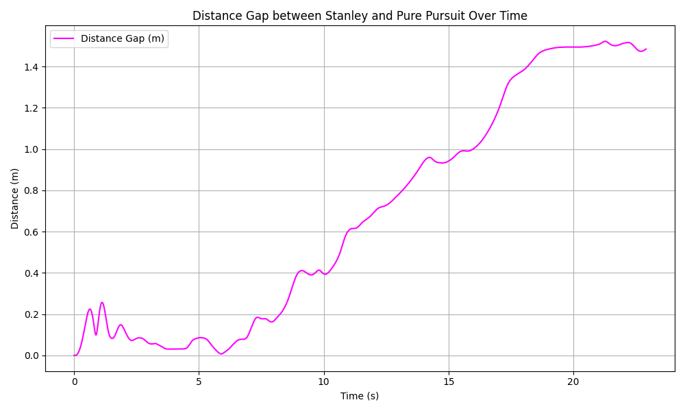
Distance Gap (Optional)

1. Track how far the car deviates from ideal path (cross-track error)

6.3 What the Results Tell Us

These graphs and metrics help answer:

1. Did our controller follow the optimized line well?
2. Did the car slow down properly in curves and speed up in straights?
3. Was Stanley smoother than Pure Pursuit?
4. Where are we losing time — poor path? poor speed profile?

This step gives you real feedback that you can use to:

1. Justify your choices
2. Tune further if needed
3. Show evidence of learning-based behavior

Output of This Step:

1. Lap time improvement
2. Side-by-side graphs of controller performance
3. Validated the impact of the optimization pipeline

To move beyond simulation and into the realm of real-world deployment, this project has been designed with ROS2 compatibility in mind. ROS2 (Robot Operating System 2) is a middleware framework widely adopted in robotics, offering modularity, scalability, and real-time communication between distributed system components.

By wrapping our optimized trajectory, speed profile, and control logic into ROS2 nodes, we enable direct deployment on real F1TENTH platforms — or any custom mobile robot.

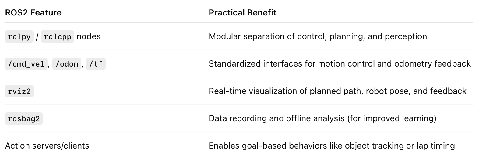
Why Integrate with ROS2?

refer the table from this section above

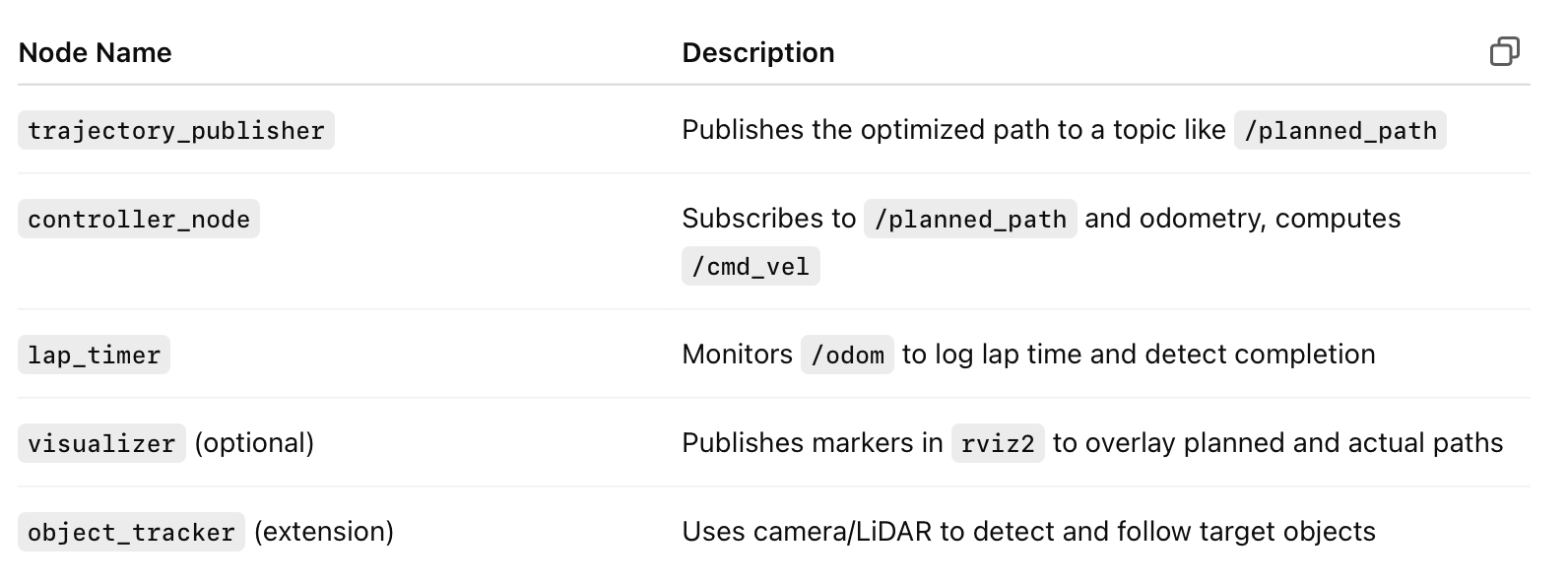
Suggested ROS2 Node Architecture

You can break your project into the following ROS2 nodes:

refer the table from this section above

Deployment Path to Physical Car

1. Convert core scripts (controller.py, optimize_speed.py) into ROS2 nodes using rclpy
2. Subscribe to real-time sensor data (e.g., /odom, /imu, /scan)
3. Publish steering and speed commands to /cmd_vel
4. Visualize live telemetry with rviz2 overlays
5. Record sessions using rosbag2 for offline trajectory refinement

Benefits of ROS2 Transition

1. Seamless integration with Jetson, RPi, or embedded hardware
2. Real-time diagnostics, tuning, and behavior tracking
3. Extensible pipeline: plug in YOLO object detection, lane tracking, or RL modules

This project demonstrates that you don’t need machine learning to build an intelligent, fast-driving racecar.

Using classical controllers, curvature-aware speed profiles, and simulation-based feedback, we already achieved significant lap time gains.

But if you want to take this to the next level — here’s where you can go.

1. Dynamic Speed Control (Online Braking & Throttle)

So far, speed was precomputed offline.

What if the car could adjust speed in real-time based on upcoming turns?

You could implement:

1. Longitudinal PID controller for dynamic acceleration/braking
2. Use lookahead curvature to slow down before sharp curves

2. Model Predictive Control (MPC)

Unlike Pure Pursuit or Stanley, MPC plans ahead using system dynamics and constraints.

Benefits:

1. Considers both position and velocity
2. Optimizes over a prediction horizon
3. More human-like driving behavior

Drawback: higher computation cost.

3. Vehicle Dynamics Modeling

Right now we assume a simplified point-mass model.

Adding a bicycle model, friction limits, or Ackermann steering constraints would:

1. Make the simulation more realistic
2. Improve generalization to physical platforms

4. Integrating Reinforcement Learning (RL)

If you're curious about RL, you can replace your controller with an end-to-end policy:

1. Input: state vector (position, heading, speed, curvature)
2. Output: steering + throttle
3. Reward: minimize lap time, penalize instability

Not easy — but very powerful with enough training.

5. Real-World Deployment with ROS2

All of your code can eventually be:

1. Ported to ROS2 nodes
2. Run on a real F1TENTH car using /cmd_vel and /odometry
3. Combined with LiDAR, vision, and lane tracking

This would allow on-car learning from actual laps — the holy grail of autonomous racing.

Suggested Reading for Future Work

1. “A Survey of Motion Planning and Control Techniques for Self-driving Urban Vehicles” – González et al.
2. “MPPI Control for Autonomous Racing” – Williams et al., ICRA 2016

Takeaway

This project lays the groundwork for intelligent autonomous driving — using interpretable, explainable techniques.

From here, you can choose your path:

1. More control theory
2. More autonomy
3. Or real-world testing and deployment